One of the primary objectives when designing software is to strive for simplicity. We are reminded of this through acronyms, adagia and our failure to easily comprehend our colleagues' — or, perhaps more often, our own — code. But what does it mean to “Keep It Simple, Stupid”? And when is software too complex?

In this post, we will explore complexity from the perspective of execution flow in our code. We will have a look at a formal, rigorous method of assessing this complexity and, even though these measures are not novel, they are still worth knowing (and trying out) when striving for quality software.

Complexity

Recently, I have been reading some of the notes of Edsger W. Dijkstra (1930 - 2002). He contributed a lot to the software engineering profession as we know it, shaping and formulizing our industry. He lived in a time where computers were becoming ubiquitous, yet programming was not largely considered as its own profession. Rather, programming was something for puzzlers, mathmaticians and (later on) computer scientists. Dijkstra realized that software engineering should be a profession of its own.

In 1970, he published his Notes on Structured Programming in which he describes the struggles of composing large programs and offers solutions by applying a disciplined, structured approach to programming called Structured Programming. With the ideas in these notes, he laid the foundation for modern software engineering and architecture.

(…)

We should recognize that already now programming is much more an intellectual challenge: the art of programming is the art of organizing complexity, of mastering multitude and avoiding its bastard chaos as effectively as possible.

(…)

[W]e can only afford to optimize (whatever that may be) provided that the program remains sufficiently manageable.

– Dijkstra (EWD249, 1970, p. 7)

Although this was 50 years ago, it is still extremely relevant today. We are still organizing complexity and battling chaos on the daily and we still need to educate our engineers on the virtues of elegant code and the perils of what we now call premature optimization.

In order to verify functional quality we can leverage (automated) testing and analyze code coverage and mutation test coverage, but how can we measure the structural quality of our code? One way of discerning this quality is by gauging its structural complexity.

Measuring Complexity

Dijkstra, among others, spearheaded a movement of formal software design through structured programming. In the same vain, attempts were made to quantify the design quality of software: empirical software engineering.

Metrics like number of files and logical lines of code were used to indicate the scale of a project but this did not necessarily say something about the complexity of the code itself. To get an insight into the complexity of code, one would need to study how difficult the code in question is to understand.

Graph-based Complexity Metrics

A program that has a varying amount of possible outcomes because of the decisions being made, is more difficult to reason about. It becomes less transparent what the impact is of a certain change and how the software behaves when given different inputs or when placed under varying conditions. Through structured programming, modularization was gaining traction as a means of organizing complexity. But when is a module too complex?

This question is at the heart of McCabe’s 1976 paper called A Complexity Measure:

What is needed, is a mathematical technique that will provide a quantative basis for modularization and allow us to identify software modules that will be difficult to test or maintain.

– McCabe, A Complexity Measure (1976), p. 1.

The mathematical approach proposed by McCabe is based on graph theory’s circuit rank or cyclomatic number.

Calculating McCabe’s cyclomatic complexity requires thinking of modules as (control flow) graphs. A program control graph requires unique entry and exit nodes, all nodes being reachable from the entry and the exit being reachable from all nodes.

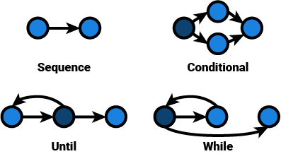
A graph consists of nodes and edges. In a program, a node can be seen as an instruction, while an edge represents control flow between the nodes. Conditional statements are then represented by branching, while iteration is expressed as revisiting nodes on a path (decisions are accented):

Cyclomatic Complexity

McCabe’s cyclomatic complexity v is calculated by taking the number of edges e and subtracting the number of nodes n. Finally, add the number of components p times two. Typically, the number of components is 1, unless one is looking at a collection of modules.

v = e - n + 2 * p

A sequence, no matter its length, has a cyclomatic complexity of 1. Imagine a sequence of 2000 nodes. It has n - 1 edges: 1999. Its cyclomatic complexity is 1: unit complexity.

v = 1999 - 2000 + 2 * 1
v = 1

Conditional statements, like the one aforementioned, have a cyclomatic complexity of 2.

v = 4 - 4 + 2 * 1
v = 2

The same goes for iteration:

v = 3 - 3 + 2 * 1
v = 2

Let’s apply this to some Python code. Imagine a function, determine_season, that determines the meteorological season for the northern hemisphere based on the number of the month (1 being January).

def determine_season(month):
    if 3 <= month <= 5:
        return "Spring"
    elif 6 <= month <= 8:
        return "Summer"
    elif 9 <= month <= 11:
        return "Autumn"
    else:
        return "Winter"

This function branches in 4 directions, one for each season:

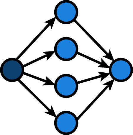
Its cyclomatic complexity is similar. We could also count all if and elif statements and add 1 to get the cyclomatic complexity.

v = 8 - 6 + 2 * 1
v = 4

Note that I only drew a single node to represent the return flow as we need a single exit node for our graph. I do not adhere to the single return philosophy popularized by most structured programmers. For cyclomatic complexity, it does not matter whether we use a variable that is initialized and assigned based on the decision in each branch and return that variable or whether we leave out the intermediate state. The exit node can be seen as the same operation: returning the value decided upon.

Myers' Extension

A critical reader may have theorized that our determine_season function may have some more decision nodes than is shown in the graph. That reader would have a point, as our if-statements actually contain a combination of conditions, even though Python obscures it a bit with its syntactic sugar:

def determine_season(month):
    if month >= 3 and month <= 5:
        return "Spring"
    elif month >= 6 and month <= 8:
        return "Summer"
    elif month >= 9 and month <= 11:
        return "Autumn"
    else:
        return "Winter"

You see? We were using logical and in disguise. And a logical and can, in turn, be functionally be seen as a nested if-statement in disguise:

def determine_season(month):
    if month >= 3 
        if month <= 5:
            return "Spring"
    elif month >= 6:
        if month <= 8:
            return "Summer"
    elif month >= 9:
        if month <= 11:
            return "Autumn"
    else:
        return "Winter"

It’s difficult to produce a flow graph of this code, because the alternative for each inner if-statement passes back control to the outer if/elif/else-statement. I might try and produce something like this:

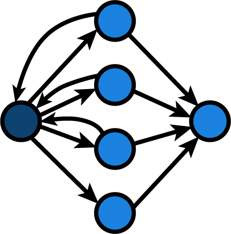
This would actually leave us with a cyclomatic complexity of 7.

v = 11 - 6 + 2 * 1
v = 7

This is one of Myers' (1977) considerations, who suggests an improvement to this calculation in his paper “Extension to Cyclomatic Measure of Program Complexity”. He argues for calculating a complexity interval of a lower bound and an upper bound instead of a single number. The lower bound would consist of the decision statement count (McCabe’s metric) and the upper bound would consist of the individual conditions + 1. In the first example of our determine_season function, Myers' cyclomatic complexity interval would be: (4:7).

Automation

Ever since complexity measures have been devised, programs have been written to automate the analysis of code against these measures.

Lizard can calculate the cyclomatic complexity for software written in various languages. It aligns closely with McCabe’s complexity, although it counts switch statements by the number of cases and looks at logical expressions for branching (Myers' correction). However, it disregards Python’s syntactic sugar. It regards 3 <= month <= 5 (1) as half as complex as month >= 3 and month <= 5 (2). Lizard offers information on lines of code, token count, parameter count and cyclometic complexity.

Another popular tool for Python is radon. Radon supports various metrics: McCabe’s complexity, raw metrics, Halstead metrics and a maintainability index (used in Visual Studio). Radon’s complexity calculation works the same as lizard’s and, likewise, it disregards Python’s syntactic sugar when doing ranged comparisons. Radon is used in Codacy and CodeFactor and can be used in Code Climate and the coala analyzer. Radon can also work as a monitoring tool in the form of Xenon.

In Java land, there are a lot of tools. One famous tool is PMD. It offers a bunch of metrics. In the complexity department it offers three flavors of cyclomatic complexity:

1. Standard Cyclomatic Complexity: McCabe’s complexity
2. Cyclomatic Complexity: McCabe’s complexity with added points per logical expression
3. Modified Cyclomatic Complexity: McCabe’s complexity, but treating switch statements as a single decision point.

Interestingly, PMD also offers metrics regarding NPath complexity, in which the amount of acyclic execution paths are measured instead of just the decision points.

PHPMD is a port of PMD but only offers Cyclomatic and NPath Complexity. It seems that PHPMD’s Cyclomatic Complexity is similar to McCabe’s with added points per logical expression.

For JavaScript, there used to be a tool called JSComplexity. It seemed to have been renamed to escomplex. Based on the source code, it looks like escomplex used McCabe’s complexity plus 1 for each logical expression.

ESLint also has the ability to check cyclomatic complexity. The documentation is unclear about how this is calculated, but the source code seems to suggest that it is McCabe’s complexity with added points per logical expression.

Perhaps the most famous tool for continous quality inspection is SonarQube. It supports multiple languages, a wide range of metrics and offers both offline tools and an online platform. With regards to complexity, they offer cyclomatic complexity and their own metric, cognitive complexity, which is supposed to be a correction on cyclometic complexity measurements by focusing more on the understandability of the code.

Critique

Cyclomatic complexity focuses on the complexity of the program control graph. This does not necessarily mean that it will adequately predict whether code is easy to understand, but it can be used as an indicator for further investigation.

Purely symmetrical if/elif/else statements, like switch statements, grow in cyclomatic complexity linearly — even though it is not hard to follow for the average programmer if the inner lines of code are short and unnested.

The same happens when applying Myers' extension. Representing combined conditions as more complex in terms of human comprehension would be inaccurate. Furthermore, nested sequences, recursive calls and pretty long sequences are often difficult to understand for humans. McCabe’s metric and its extensions do not sufficiently account for that. Other metrics, like Nejmeh’s NPath complexity regarding the amount of possible paths, from start to exit, that can be taken in a certain module could prove more insightful in this regard. Similarly, metrics like Sonar’s Cognitive Complexity, which specifically focuses on measuring the understandability of source code can be an interesting data point to study. Perhaps we will explore these in a later blog post.

Besides Myers', several attempts have been made to amend McCabe’s metric. For example, Hansen (1978) proposed counting conditions, function calls, iterations and logical expressions, but counting a switch/case statement only once because they are easier to understand. For an extensive critique on cyclomatic complexity as a software metric, see Shepperd’s 1988 paper on the subject.

Another point of discussion is whether the calculations should apply to any programming paradigm or style. Functional, reactive, event-driven paradigms and styles typically use different flow constructs than their imperative counterparts. It can even be debated whether the metric is as useful for object-oriented code. Either way, the cyclomatic complexity can be calculated; the treshold for what is considered acceptable or not shall differ per project, language and paradigm.

That being said, the calculation of cyclomatic complexity still proves its usefulness – even though automated calculations seem to calculate it differently. The metric, especially when corrected by Myers' extension, indicates the upperbound for the amount of linear paths that need to be tested. This does not necessarily mean that each path requires a separate test. At least the amount of input variations and assertions against the output should match the (corrected) cyclomatic complexity.

In conclusion

I think it is in society’s best interest to reduce the complexity of the software we create. It is what distinguishes a good programmer from a great one. We need to set aside our ego’s and strive for continuous improvement through honest feedback and measured results. Again, I think Dijkstra said it best. In his ACM Turing Lecture of 1972, the Humble Programmer, he exclaimed:

“(…) The competent programmer is fully aware of the strictly limited size of his own skull; therefore he approaches the programming task in full humility, and among other things he avoids clever tricks like the plague. (…)”

– Dijkstra (EWD340, 1972)

Continuously assessing the quality of our work can help us stay a humble programmer. Code metrics can play an important role in this.

Quality measures can help our team find out which lines of code need to be made more elegant and simple, which lines are in need of more extensive testing and of which lines we can be proud. One such measure, although imperfect and ambiguous, is cyclomatic complexity. Even though the metric does not directly lead to a conclusion about the quality of our code, it can help us identify the areas that need some work. Perhaps in a later blog post, we will explore other (complexity) metrics.